Leverage Calculation And Approximation for Large Scale ℓ1-Norm Data Analysis
Salvador A. Flores
*S. Flores is with the Mathematics Engineering Department and the Center for Mathematical Modelling, Universidad de Chile, Chile. e-mail: sflores@dim.uchile.cl
Abstract Identifying influential observations is a fundamental task in data analysis. It has served longtime to detect outliers and other deviating behaviors in data. Presently, it is having an essential role in the development of techniques for obtaining coresets to reduce huge amounts of data to smaller, manageable ones with provable warranties. For least squares regression, the subject is well understood both in the theoretical and computational setting. Other estimation techniques, such as ℓ1-norm minimization, have several advantages over least squares in terms of robustness and identification of influential observations, but diagnostics are not developed enough, which hinders extensions of these methods to large scale data. In this paper we study the proper definition and numerical estimation of leverage scores for ℓ1-norm minimization. We show that the calculation of ℓ1-norm leverage scores amounts to solving a linear programming problem. In view of applications to big data analysis, this raises the issue of the trade-off between computing exact or very good quality leverage scores, at a high cost, versus using fast approximations to obtain raw approximations. Based on this linear programming formulation, we compare the quality of approximated leverage scores proposed in the literature with respect to the exact ones. We also propose a randomized approximation which is included in this evaluation. Additionally, we use linear programming duality to derive several of approximations to the exact leverage scores, with different levels of quality and complexity.
Consider the classical linear regression model, where each observation yi follows
|
| (1) |
for some parameter β ∈ℝp to be estimated, where the xi ∈ℝp are the corresponding vector of independent variables or carriers and δi are random deviations from the model. It is customary to assume i.i.d errors, and in many cases it is implicitly assumed that errors behave like Gaussian random variables.
Regression diagnostics are essential in helping data analysts to identify failures of the assumptions that customarily accompany regression models. Most of them look for evaluating the impact of each datum on the estimated coefficients, the predicted (fitted) values or the residuals. The concept of leverage holds a prominent place in regression diagnostics. For instance, in Least Squares (LS) regression, they correspond to the diagonal element hii of the ”hat” matrix H = X(X⊤X)-1X⊤. These quantities can be efficiently computed and enjoy a bundle of properties, most of them stemming from the linearity of the estimation of fitted values.
The ℓ1 estimator, also called Least Absolute Deviations (LAD), is defined as a solution to
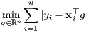 | (2) |
This estimator is distinguished for its robustness to outliers. Nonetheless, for many years the non-differentiability of the objective function complicated the use of LAD regression, delaying the development of regression diagnostics. The emergence of mature implementations of linear programming algorithms made the calculation of LAD estimates possible for data in the order of hundreds of thousands [1]. Also, specific algorithms for computing the effect of adding or removing observations from the LAD fit have appeared since then [2, 3, 4] which have contributed to close the gap between LAD and LS concerning row deletion methods [5]. Surprisingly, even if leverage has been defined for LAD regression by [?] in 1992, its computation has not been treated yet, and contrarily to LS leverages, is not included in any statistical package or library.
Recently, the increasing need for big data regression has renewed the interest in leverage calculations [6, 7] for LAD regression. As opposed to what is done in robust regression, these methods favour high-leverage observations, since few of them mostly determine the LS fit. In this way, performing regression in an properly sampled sub population (a coreset or sketch) provides an accurate approximation to the “true” estimator, reducing considerably the size of the numerical problem when n is huge [8]. [9] devised an algorithm to compute the leverage scores without computing pseudo-inverse matrices. They also point out interesting applications of maximum leverage values to problems such as identifying important nodes in a network or very small clusters in noisy data, among others. Concerning robustness, there has been some attemps to extend these sampling techniques to LAD regression [10] and more generally to quantile regression [11].
Our goal is to compute leverage scores as a data exploration tool in a context broader than just approximating the LAD regression estimator. Obviously, the task being harder, at first implies restricting to smaller problems and/or been ready to increase the devoted computational resources. However, we are deeply convinced that the rapid development both in High Performance Computing (HPC) and in theory and algorithms will shortly make the use of regression diagnostics routine even for very large scale data. We aim at contributing in that direction.
Our contributions are:
In Section II we discuss the best notion of leverage to adopt for this study. Then, in Section III we derive the linear programming formulation of LAD leverages, and derive some bounds using duality theory. The randomized approximation is desbribed in Section IV. Section V is devoted to a preliminary numerical evaluation of the accuracy of some approximations to LAD leverage scores. Finally, we close the paper with a few conclusions and a lot of avenues of continuation of this work, presented in Section VI.
II. Leverage, sensitivity and related concepts
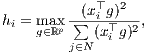
The concept of leverage is central in regression diagnostics. In LS regression, it corresponds to the diagonal element hi ≡ hii of the projector onto the range of X, called hat matrix:
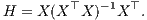 | (3) |
Alternatively, if U is any orthonormal basis of the column space of X, then
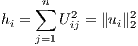 | (4) |
where ui is the i-th row of U. Equation (4) has been used [10, 8] to extend the notions of leverage to ℓ1 norm by using the leverage proxies
 | (5) |
as a by-step to devise sampling algorithms. Despite the numerical ease in computing such quantities, there are no associated theoretical properties providing sustenance to such a definition. Nonetheless, this definition worked well for their objective, approximating the LAD estimator by sampling, which is different from ours.
Yet another equivalent expression for (3) is:
 | (6) |
derived in [12] and used as a departing point to extend the notion of leverage in at least two directions, by making possible to define leverage for groups of observations and for more general estimation techniques than LS. For i = 1,...,n, we shall denote by γi the individual leverage of observation i, given by
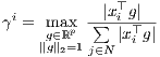 | (7) |
There are results in two key application fields where this definition stands out as the most adequate one:
One of the main reasons for using ℓ1-norm in regression is its resistance to outliers. Both [13] and [12] have stablished the links between the leverage indicator γi and the robutness properties of LAD regression to outliers. Later, [14] proved, for data perturbed by noise and outliers and as long as γi < 1∕2, that the regression fit differs from the fit without outliers proportionally to the noise amplified by a factor (1∕2 - γi)-1, independently of the outliers magnitude. This result extends to group of observations as well.
An strategy for processing large amounts of data consists in creating a tractable summary of the data, called coreset or sketch, which, for an specific analysis, gives results that are provably close to those obtained on the whole dataset. This data reduction technique is known as Sketching. In practice, sketching is performed by sampling data according to some particular distribution that favors points of high relevance for the analysis in mind. For LS regression, the sampling distribution is proportional to hi∕p. In the broader context of constructing coresets for Empirical Risk Minimization (ERM) problems,
 | (8) |
by random sampling, [15] shows that while bias can be corrected by a proper re-weighting, in order to minimize the variance of the sampled cost function each point has to be drawn with probability proportional to:
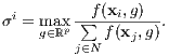 | (9) |
Note that the expression in (9) needs, in many cases, a normalization in order to be well-defined. When the function f is homogeneous
in g for instance, the solution is unique up to scale. This framework encompasses linear, quantile and logistic regression, support vector
machine, clustering and many other machine learning problems. In particular, for a slightly modified version of LAD regression we
recover the expression for leverage (7).
Despite its appealing theoretical properties, and even if we are going to show next that they can be formulated as efficiently solvable linear programs, this leverage scores are not amenable for computation at scale. For this reason, in what follows we aim at obtaining ways to approximate them and evaluate the quality of different approximations in tractable instances of the problem.
III. Computing leverage indicators for LAD regression by Linear Programming
The leverage definition (7) has good theoretical properties, but in general is a difficult optimization problem involving a non-convex objective function. As a first step towards deriving good approximations, we show that those optimization problems can be cast as linear programs. The advantages are twofold. First, it allows to compute leverage scores for medium-sized problems, which can be used to understand and assess the quality of any proposed approximation in small problems. Secondly, we have at our disposal the battery of results on linear programming to exploit.
proof
The key observation to cast (7) as a LP is that |xi⊤g|∕∥Xg∥1 is invariant with respect to scale changes of g, therefore the
normalization ∥g∥2 = 1 can be replaced by any other, such as ∥Xg∥1 = 1, as long as it is not degenerate, which is
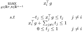
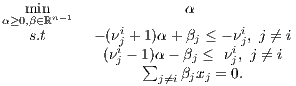
the case here since X has full rank. Therefore the constants γi can be evaluated by solving the convex optimization
problem
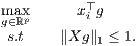 | (10) |
Note that the constraint ∥Xg∥1 ≤ 1 will always hold as equality at the optimum, since ∥Xg∥1 contains the term |xi⊤g| which is being
maximized. Problem (10) is equivalent to (Pi). To see this, rewrite the constraints -tj ≤ xj⊤g ≤ tj equivalently as |xj⊤g|≤ tj. Then,
xi⊤g + ∑
j≠itj ≤ 1 amounts to ∥Xg∥1 ≤ 1, given that the term xi⊤g being maximized must be positive at the optimum, and that
|xj⊤g| = tj for j≠i, at the optimum too. We have established that Value(Pi) = γi.
A strong consequence of the linear programming formulation is duality theory. For any linear program in primal form minc⊤x : Ax = b,x ≥ 0 we can associate a dual linear problem of the form maxb⊤y : A⊤y ≤ c. The so-called weak duality theorem ensures that for any primal feasible point x and dual feasible y, it holds

Theorem 2: Let hij denote the entries of the hat matrix H = X(X⊤X)-1X⊤, and define
 | (11) |
Consider the following linear programs
 | (Di) |
The following hold:

proof
We show that the optimization problem (7) can be cast as a linear program, and the claimed relations will follow as consequence of LP
duality.
Let us show that (Di) is the dual problem to (Pi). By definition, the linear dual to (Pi) is
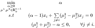 | (12) |
Notice that μj1 and μj2 are Lagrange multipliers of xj⊤g ≤ tj and -tj ≤ xj⊤g ≤ tj, respectively, therefore they cannot take a non-zero value simultaneously. For this reason we can simplify problem (12) by defining μ := μ1 -μ2. In this way, μj1 -μj2 = μj and μj1 + μj2 = |μj|, yielding
 | (13) |
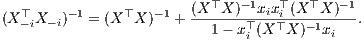
In order to proceed to further simplications of (13) it will be convenient to introduce the notation X-i for the (n - 1) × p matrix obtained by supressing the ith row of X. Consider the orthogonal decomposition μ = X-iθ + β, with β ∈ kerX-i⊤. From the first equation in (13),
| νji | = x j⊤(X -i⊤X -i)-1x i | (14) |
= xj⊤(X⊤X)-1x
i +  | (15) | |
= hji +  | (16) | |
=  | (17) |
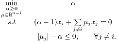
As a consequence, those μ ∈ℝn-1 satisfying (α- 1)xi + ∑ j≠iμjxj = 0 can be parameterized as μ = {(1 -α)νi + β ∣β ∈ kerX-i⊤}, which replaced in (13) yields to (Di). The equality γi = Value(Di) is therefore a direct application of the strong duality theorem for linear programming, using the fact Value(Pi) = γi proved before. Note that li is the value of (Pi) for the feasible point g = xi∕∥Xxi∥1, therefore li ≤ max(Pi). Similarly, considering only feasible points with β = 0 in (Di),
 | (18) |
and since maxj≠i|νji|∕(1 + |νji|) = ui, the result follows from the fact that restricting the feasible domain of a minimization problem
can only increase its optimal value.
Note that in the previous result we make only an elementary use of LP duality, considering primal points with a large portion set to zero. Further analysis may lead to tighter upper and lower bounds. The challenge in doing so is to find a good balance between the improvement of the approximation versus the increase in the time to compute it. Therefore, this Theorem should be considered only as a starting point rather than as a definitive result.
IV. Distributed randomized leverage scores estimation
A drawback of the approximations presented so far is that in general they need all the data to make calculations, such as solving a LP problem or compute the SVD decomposition. Though, very large volumes of data are customarily stored in distributed systems, which makes difficult to operate over the whole data at once. Another point to stress is that the definition of leverage changes very mildly from one observation to another. All of them carry the term ∥Xg∥1 on the denominator, for instance. If instead of optimizing over the whole sphere we computed the maximum over a finite set of directions g1,...,gk,...,gm, we could compute only once, locally at the node I where the datum xi is, the terms |xi⊤gk|, saving communication burden among nodes by broadcasting only the real numbers ∥XIgk∥1 instead of the whole data XI. With this information, each node forms the common term ∥Xgk∥1 = ∑ ∥XIgk∥1 and then computes maxk|xi⊤gk|∕∥Xgk∥1 for the points stored at that node.
 := maxk=1,...,Kqik to machine
1
:= maxk=1,...,Kqik to machine
1
 for every i = 1,...,n.
Two crucial points in the previous Algorithm are fixing the number K of approximation samples, and we way of drawing them. These questions are interrelated. A deterministic alternative is to fix and error goal ϵ and then construct an ϵ-net covering the unit sphere.
The communication costs of the Algorithm are very low, for the only vectors that are communicated are the g’s at the beginning. The rest of the time only real number are transmitted.
It is well known that the difficulty of approximating leverage values, even for LS, is higher when those are highly non homogeneous. From equation (7) we can identify the factors determining the leverage patterns:
 Fig. 1. Above: isotropically distributed points, below: anisotropic distribution, with isolated points achieving a high leverage.
For all the above reasons, we use the Bingham distribution to draw the vectors xi. This is an antipodally symmetric anisotropic probability on the sphere. In this way we can control the effect of anisotropy on the leverage distribution though the covariance structure characterizing the distribution. In order to simulate vectors of different magnitude, such as outliers, we multiply the vectors drawn from the Bingham distribution by a Cauchy random variable of location one and two scales, 0.1 and 0.15. For each combination we draw 1000 matrices and compute their exact leverage scores by solving the linear programs (Pi). Our intuition on the resulting leverage pattern is confirmed by the plots over the 100 repetitions, shown in Figure 2.
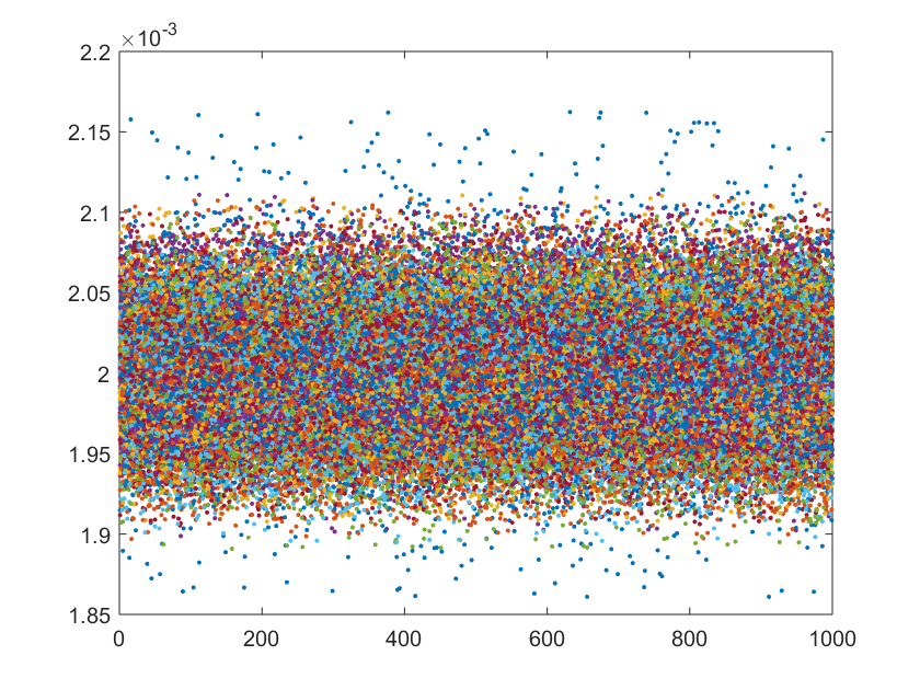
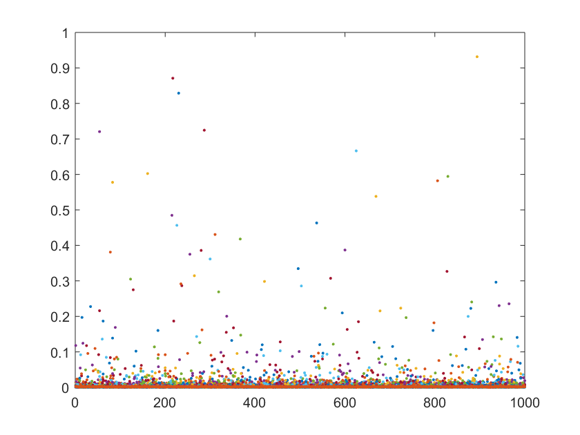 Fig. 2. Above: leverage pattern for isotropically distributed point; below: leverage pattern for anisotropic distribution containing outliers