Practical Work 1 : Fisheries models

Preliminaries : This Practical Work uses version 3.0 of the scientific software Scilab , developed by INRIA and ENPC. All the installation files can be downloaded freely from the web page http://www.scilab.org.

The PW needs two Scilab command files simu1.sce and simu2.sce, that one should store in his working directory.

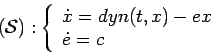
The aim of the PW is to study different harvesting policies of a stock of a renewable resource. More precisely, we consider a population dynamics, whose stock follows a natural logistic growth law and is harvested (by catches, picking, ...). The dynamical evolution of the stock can be written with the help of a ordinary differential equation :

$$\frac{dx(t)}{dt} = f(x(t)) - u(t)$$

• The state $x(t)$ of the system is the quantity of the stock at time $t$.
• The control $u(t)$ is the instantaneous speed of harvest at time $t$.

In order to simulate the solutions of the system under Scilab , let us start by defining the dynamics and the control, with the help of two functions $dyn()$ and $har()$ :

1. For the logistic law :

$$x \to rx\left(1-\frac{x}{K}\right),$$

define the function $dyn()$ as follows :
deff('[y]=dyn(t,x)','y=r*x*(1-x/K)');
and give values to the constants $r$ (intrinsic growth rate) and $K$ (carrying capacity), for instance
r=1; K=1;

2. For the control, begin by a simple law : a constant policy, as long as the stock is non empty :
deff('[u]=har(t,x)','if x>0 then u=H; else u=0; end');
and choose a value for the constant $H$, say
H=0.24;

For launching the simulations, enter the following instruction
exec("simu1.sce");
Then, a window appears :

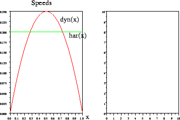
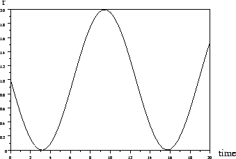
In the left, the graphs of the functions $dyn$ and $har$ are plotted. Clicking on the LEFT figure launches on the RIGHT figure the simulation of the trajectory of the dynamical system

$$\dot{x} = dyn(t,x)-har(t,x)$$

for the initial condition $x(0)$, chosen to be the abscissa of the mouse position while clicking :

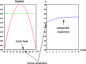
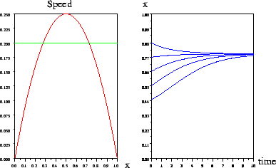
Further clicks will make different trajectories of the system superposing :

Question 1 : Study the stability of the two non-null equilibria. What is the value $x_{e}$ of the stock at the stable equilibrium ?

Question 2 : Redefine the control law $har()$ such that there exists only on non null equilibrium $x_{e}$, and such that from any non null initial condition, the trajectory converges asymptotically towards $x_{e}$. Denote
x_e=0.6;

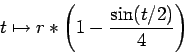
Question 3 : We consider here that the intrinsic growth rate $r$ fluctuates with time in the following manner :

$$t \mapsto r*\left(1-\frac{\sin(t/2)}{4}\right)$$

whose graph is :

Modify the function $dyn()$ to take into account this new feature, and simulate the behavior of the system for different initial conditions, and the two previous control laws. What can be concluded ?

We call harvesting effort the measure of the means available for the captures (fishermen numbers, size and number of nets, ...). We shall assume that the harvesting speed $u(t)$ is proportional to the stock $x(t)$ and the effort $e(t)$ at any time t :

$$u(t) = qx(t)e(), \qquad t \geq 0$$

where $q$ is a positive parameter, usually called capturability. At the price of renormalizing the effort $e(t)$, we can take without loss of generality $q=1$.

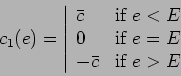
We consider now an exploitation controlled by the variations of the harvesting effort :

$$({\cal S}) : \left\{\begin{array}{l} \dot{x} = dyn(t,x) -ex\\ \dot{e} = c \end{array}\right.$$

The state of the system is now 2-dimensional, written $X$ (in caps) :

$$X=\left(\begin{array}{c} x e \end{array}\right)$$

The new control variable $c()$ is constrained as follows :

$$({\cal C}) : c(t) \in \left\vert\begin{array}{ll} \left[-\ba... ...ft[-\bar c,0\right] & \mbox{ if } e=e_{max} \end{array}\right.$$

Question 4 : Prove that for such control laws, the domain

$${\cal D} = \left\{ \left(\begin{array}{c}x e \end{array}\right) \vert x \in [0,K], \; e \in [0,e_{max}] \right\}$$

is invariant under the dynamics $({\cal S})$.

We study now possible control laws which fulfill the constraints $({\cal C})$ and stabilize the system $({\cal S})$ about $(x_{e},E)$. Three laws are considered :

1. The so-called bang-bang control :
   
   $$c_{1}(e) = \left\vert\begin{array}{ll} \bar c & \mbox{if } e... ...x{if } e = E \\ -\bar c & \mbox{if } e > E \end{array}\right.$$
   
   

2. The control linear w.r.t. $e$ :
   
   $$c_{2}(e)=\mbox{sat}_{[-\bar c,\bar c]}(G(e-E))$$
   
   

3. The state feedback law :
   
   $$c_{3}(x,e)=\mbox{sat}_{[-\bar c,\bar c]}(G_{1}(x-x_{e})+G_{2}(e-E))$$
   
   

where $G$, $G_{1}$ and $G_{2}$ are tuning parameters, and $sat$ is the saturation function :

$$\mbox{sat}_{[m,M]} : \xi \to \left\vert\begin{array}{ll} M &... ... \xi \in [m,M]\\ m & \mbox{if } \xi \leq m \end{array}\right.$$

Define
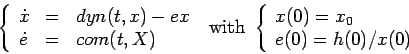
H=0.24;x_e=0.6;E=H/x_e;cbar=0.1;

For the simulations, consider that $r$ is again constant, which amounts to define the dynamics as follows :
deff('[y]=dyn(t,x)','y=r*x*(1-x/K)');

The control law is defined in Scilab with the help of the function $com()$. For instance, for the ``bang-bang'' law :
epsilon=1e-3;
deff('[edot]=com(t,X)','e=X(2);..
if abs(e-E)< epsilon then edot=0;..
else edot=cbar*sign(E-e); end');

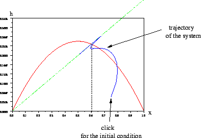
Simulations are launched entering the instruction
exec("simu2.sce");
A window then appears :

A click in the window chooses an initial condition $(x_{0},h_{0})$, computes and represents the generated trajectory of the system

$$\left\{\begin{array}{lll} \dot{x} & = & dyn(t,x)-ex\\ \dot{... ...begin{array}{l} x(0)=x_{0} e(0)=h(0)/x(0) \end{array}\right.$$

The trajectory is drawn in the plane $(x,h)$ with $h=xe$.

Question 5 : Simulate the control law $c_{1}$. What happens if one takes epsilon=0 ?

Question 6 : Write in Scilab the control law $c_{2}$, and simulate the trajectories taking different values of the gain $G$ between $-0.01$ and $-0.1$. Explain the qualitative behaviors ?

Question 7 : Write in Scilab the control law $c_{3}$, and simulate the trajectories taking different values of the gains $G_{1}$ and $G_{2}$. Determine analytically the pairs $(G_{1},G_{2})$ insuring a local asymptotic stability of the closed loop system.

With the option :
linearise='on';
activated, entering the instruction exec("simu2.sce"); computes and draws (in dashed lines) in addition the trajectory of the system $({\cal S})$ linearized about $(x_{e},E)$, in the plane $(x,h)$ :

Question 8 : Launch gain the simulations of the different control laws, together with the drawing of the trajectories of the linearized dynamics What can be concluded ?

END

Practical Work sheet prepared by Pierre Cartigny and Alain Rapaport.